What is Spatial Autocorrelation
Spatial autocorrelation measures the variation of a variable by taking an observation and seeing how similar or different it is compared to other observations within its neighborhood [1]. In other words, it measures wether and how much nearby observations influence each other.
In real estate, properties close to each other often whare similar characteristics (e.g. neighborhood quality, amenities) and thus may have similar prices.
Interpretation
Similar to traditional correlation measures, spatial autocorrelation values go from -1 to 1. Positive spatial autocorrelation results when observations within a neighborhood have similar values, either high-high (HH) values or low-low (LL) values. Negative spatial autocorrelation is a result of having low values next to high values, or viceversa. [1]
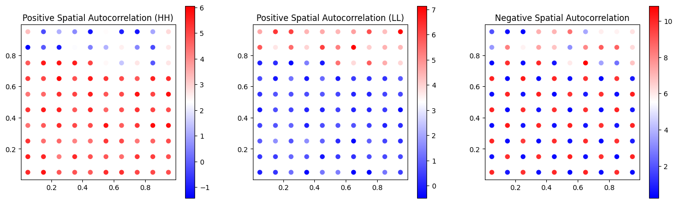
In the figure above, we can see three sets of data.
- The first has a high value cluster in the bottom and a lower value cluster in the top. Since most of the points are high values, it would return a HH positive spatial autocorrelation.
- The second set of data is the same but inverted, more lower values, therefore it would have a LL positive autocorrelation
- The third one has low values surrounded by high values (and the other way around), so it would return a negative spatial autocorrelation and, depending on the number of Low-High (LH) and High-Low (HL) relationships, it would return one of them.
Global and local spatial autocorrelation
Spatial autocorrelation is measured in 2 ways: Global and Local.
Global: Measures the trend in an overall dataset, it helps to understand the degree of spatial clustering present.
Local: Measures the localized variation in the dataset and helps detect the presence of hot spots or cold spots
- Hot spots: Localized area clustes with statistically significant high values
- Cold spots Localized area clustes with statistically significant lower values
Spatial weights
To define the neighborhood of a given observation (i.e. in the real estate data, which are the properties considered ’neighbors’ of another), spatial weights matrices are used. There are three main spatial weights matrices: rook contiguity matrix, queen contiguity matrix and K-Nearest Neighbors (KNN) matrix.
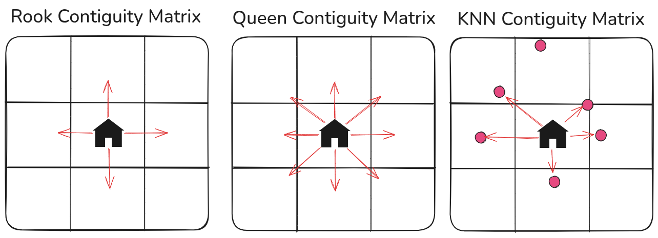
Rook contiguity matrix
- Takes the four nearest neighbors in a north (N), south (S), east (E), and west (W) direction.
- Named after the rook chess pice since it follows the same directions.
Queen contiguity matrix
- Takes the eight nearest neighbors in N, NE, NW, S, SE, SW, W and E directions
- In a similar fashion to how a queen moves about a chessboard.
K-Nearest Neighbors (KNN)
- Takes the closest $k$ neighbors in any direction.
- Uses the Euclidean distance
The weight is used for the spatial autocorrelation testings and depending on the used matrix it could yield different results.
Spatial lags
A spatial lag is a byproduct of the spatial weights matrix. A spatial lag is a variable that averages the values of the nearest neighbors, as defined by the spatial weights matrix chosen.
For example, in real estate, the spatial lag of a property using KNN (k=5) when we’re interested in the selling price would be the average selling price of the 5 closest properties.
Testing for Spatial Autocorrelation
The measures (test statistics) related to the existence of global and local spatial autocorrelation in data are defined as:
- Global indicators of spatial association (GISA)
- Local indicators of spatial association (LISA):
Testing for Global Spatial Autocorrelation
The most common measures used to test the existence of spatial autocorrelation [2] in the data are Moran’s I [3] and Geary’s C [4]. The null and alternative hypotheses for these tests are [1]:
- $H_0$: The data is distributed randomly across space
- $H_a$: The data exhibits a spatial structure and is not randomly distributed
Monran’s I
$$Moran’s\ I = \frac{N}{S_0} \frac{\sum_{i=1}^{N}\sum_{j=1}^{N} w(i,j)(x_i - \bar{x})(x_j - \bar{x})}{\sum_{i=1}^{N}(x_i - \bar{x})^2}$$
Where:
- $(x_i - \bar{x})$: the standardized value of the variable of interest (voi)
- $(x_j - \bar{x})$: the standardized value of the lag of the voi
- $\bar{x}$: mean of the voi
- $N$: number of features
- $S_0$ the aggregate of spatial weights
Moran’s I ranges from -1 to +1. A positive value indicates positive spatial autocorrelation and a negative value indicates negative spatial autocorrelation. Values near zero suggest a random spatial pattern.
Geary’s C
$$Geary’s\ C = \frac{(N-1)}{2S_0} \frac{\sum_{i=1}^{N}\sum_{j=1}^{N} w(i,j)(x_i - x_j)}{\sum_{i=1}^{N}(x_i - \bar{x})^2}$$
Geary’s C ranges from 0 to 2. A value less than 1 indicates positive spatial autocorrelation, a value greater than 1 indicates negative spatial autocorrelation, and a value of 1 suggests a rnadom spatial pattern.
Statistics for Local Spatial Autocorrelation
Local spatial autocorrelation measures the relationship between each observation and its localized surroundings. Compared to global spatial autocorrelation, local spatial autocorrelation does not return a single value but instead returns values per observation.
Local Indicators of Spatial Associations (LISAs) are spatial statistics that are derived from global spatial statistics and calculate local cluster pattern, also known as spatial outliers.
Similar to the GISAs, there is a Local Moran statistic and a Local Geary statistic [5].
Local Moran’s I
$$I_i = \frac{x_i - \bar{y}}{m_2} \sum_{j} w(i,j)(x_j - \bar{x})$$
Where
- $m_2$ is a constant defined as $m_2 = N^{-1} \sum_{i}(x_i - \bar{x})$
- $(x_i - \bar{x})$: the standardized value of the variable of interest (voi)
- $(x_j - \bar{x})$: the standardized value of the lag of the voi
- $\bar{x}$: mean of the voi
- $N$: number of features
Local Geary’s C
$$C_i = \frac{1}{m_2} \sum_{j} w(i,j)(x_i - x_j)$$
Spatial Autocorrelation in Guadalajara
Now moving on to the Guadalajara and Zapopan properties dataset. We will test global and local spatial autocorrelation for the following variables: price per m² (target variable), number of bedrooms, parking spaces, pool (yes/no), number of full and half bathrooms, property age, type (appartment/house).
Global Spatial Autocorrelation
The following tables shows the results of the Global Spatial Autocorrelation tests using a KNN (k=5) based matrix.
| Variable | Morans I | Morans p-value | Gearys C | Gearys p-value |
|---|---|---|---|---|
| price_per_m2 | 0.562456 | 0.001 | 0.434739 | 0.001 |
| bedrooms | 0.265306 | 0.001 | 0.729518 | 0.001 |
| parking_spaces | 0.447566 | 0.001 | 0.548583 | 0.001 |
| pool | 0.309398 | 0.001 | 0.697403 | 0.001 |
| full_bathroom | 0.382512 | 0.001 | 0.605439 | 0.001 |
| half_bathroom | 0.185348 | 0.001 | 0.803326 | 0.001 |
| property_age | 0.236803 | 0.001 | 0.736967 | 0.001 |
| gated_community | 0.476967 | 0.001 | 0.520659 | 0.001 |
| type_Appartment | 0.522861 | 0.001 | 0.480085 | 0.001 |
For each of the statistics calculated, all variables exhibited a spatial structure that is statistically significant, as shown in the table.
The plot below shows the Moran’s I statistic for the properites in Guadalajara and Zapopan. Each point represents a property and it’s relationship with the 5 nearest properties (spatial lag).
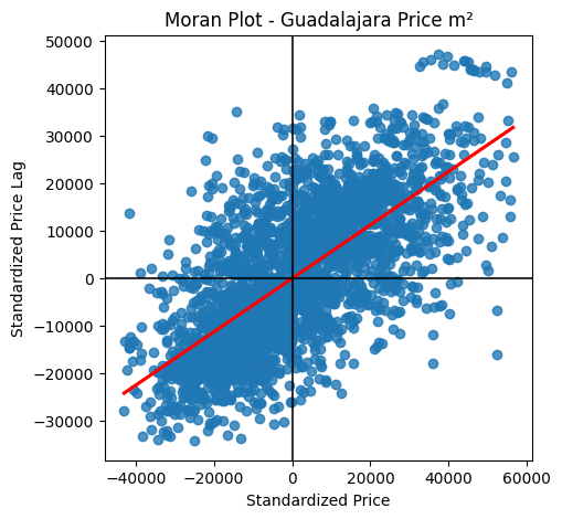
The points in the upper right quadrant have positive spatial autocorrelation, while the points in the lower left quadrant have negative spatial autocorrelation. A line of best fit, shaded red, is overlayed on the plot to show the strength of the relationship. Here, the relationship appears to be reasonably strong, as the points are distributed above and below the line of best fit to roughly the same degree.
Local Spatial Autocorrelation
Here, the LISA for the price variable was calculated using the Local Moran’s I statistic. This means that the Moran’s I was calculated for each point of the dataset with a KNN (k=5) based matrix. In the image below we can see the distribution of the Moran’s I Local test results:
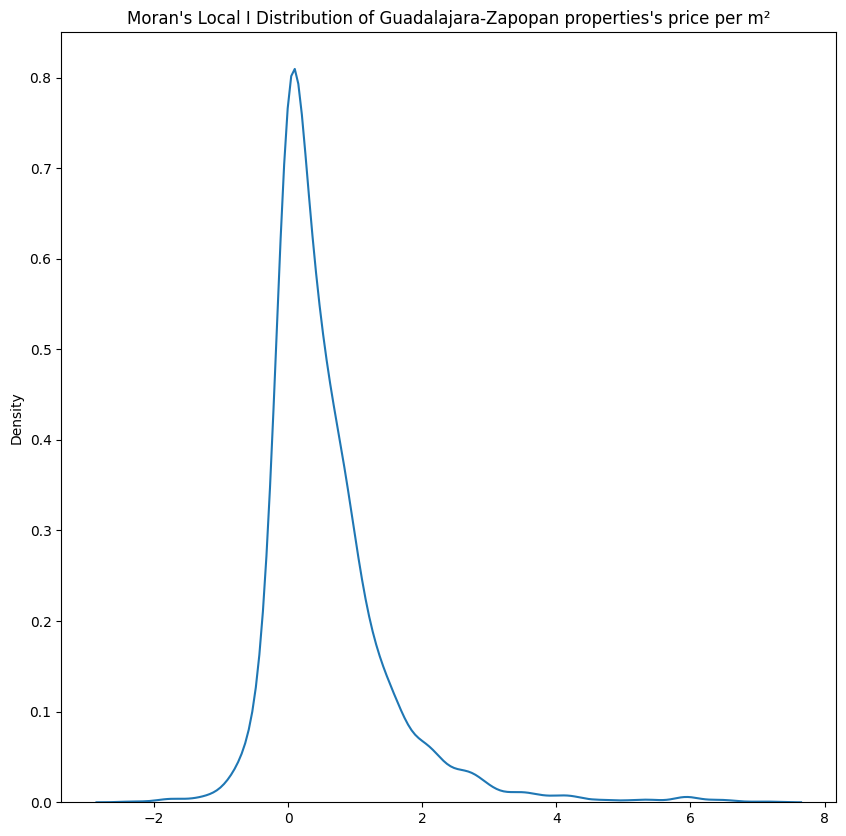
From the distribution, we can see that there is a massive spike in the data around 0 with a long right tail. This is mainly due to the presence of a large number of observations with positive spatial autocorrelation, which is in line with what we discovered from the global measures.
LISA Clusters by Neighborhood
Finally, the LISA results were used to visualize if:
- There exists statistically significant spatial autocorrelation within the properties of each neighborhood and
- What quadrant (HH, LL, HL, LH) do these properties belong in their majority
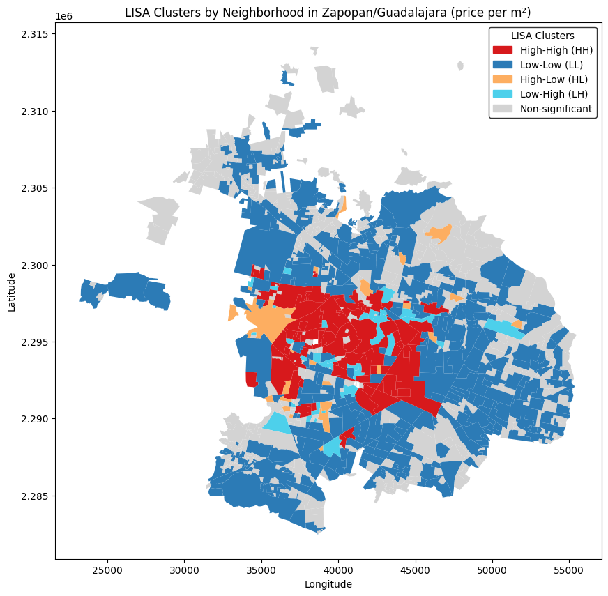
The map above, shows the neighborhoods where there exist a concentration of HH, HL, LH and LL clusters based on the price per m².
- It can be seen that there are areas without any significant spatial autocorrelation (grey),
- but that there are neighborhoods where most of the properties have either high (HH) prices or low (LL) prices and, between them,
- neighborhoods that have both Low and High properties.
- In yellow are the neighborhoods where there are more High-priced (HL) properties and
- in light blue neighborhoods where there are more Low-priced (LH) properties.
Conclusion
Guadalajara and Zapopan properties exhibit spatial autocorrelation in their price per m²: with HH clusters from West to East in the center of the metropolitan area and LL clusters in the outskirts; along with some neighborhoods in between with either LL or HL clusters.
Besides the price per m², the other variables also are significantly spatially autocorrelated, which indicates that similar houses (in size, age and characteristics) tend to be clustered around certain areas.
This has to be taken into consideration when choosing and fitting a Machine Learning model, since traditional models such as linear regression will return biased results. Models that can incorporate spatial proximity features have to be used instead.
References
[1] Jordan, D. S. (2023). Applied Geospatial Data Science with Python: Leverage Geospatial Data Analysis and Modeling to Find Unique Solutions to Environmental Problems. Packt Publishing.[2] Yamagata, Y., & Seya, H. (Eds.). (2019). Spatial Analysis Using Big Data: Methods and Urban Applications. Elsevier Science.
[3] Moran, P.A.P. (1948, July). The interpretation of statistical maps. Journal of the Royal Statistical Society B ., 10(2), 243-251. https://doi.org/10.1111/j.2517-6161.1948.tb00012.x
[4] Geary, R. C. (n.d.). The contiguity ratio and statistical mapping. The Incorporated Statistician, 5(3), 115-145. https://doi.org/10.2307/29866452517-6161.1948.tb00012.x
[5] Anselin, L. (1995). Local indicators of spatial association–LISA. Geographical Analysis, 27(2), 93-115. https://doi.org/10.1111/j.1538-4632.1995.tb00338.x